Attention in Sequence-to-Sequence Models

Overview

This study combines attention derivations with a recurrent sequence-to-sequence experiment on Multi30k. The implementation uses a bidirectional GRU encoder and a GRU decoder, rather than a full Transformer.

The main questions are when attention can select one value, when it can average two values, and how changing key magnitudes changes that behavior.

Attention weights and selection

For a query $\mathbf q\in\mathbb R^{1\times d}$, keys $\mathbf k_i\in\mathbb R^{1\times d}$, and values $\mathbf v_i\in\mathbb R^{1\times d_v}$, define

$$s_i=\frac{\mathbf q\mathbf k_i^\top}{\sqrt d},\qquad \alpha_i=\frac{\exp(s_i)}{\sum_{j=1}^m\exp(s_j)},\qquad \mathbf a=\sum_{i=1}^m\alpha_i\mathbf v_i.$$

The weights are positive and sum to one. Finite, unmasked logits do not produce exact zero or one weights. The formulation follows Vaswani et al..

Selecting one value

A sufficient condition for $\mathbf a\approx\mathbf v_j$ is $\alpha_j\approx1$:

$$\alpha_j=\frac{1}{1+\sum_{i\ne j}\exp(s_i-s_j)}.$$

The target score must dominate the combined contribution of the others. A large key norm alone does not guarantee this; its alignment with the query matters.

Averaging two values

Suppose the keys are orthonormal: $\mathbf k_i\mathbf k_j^\top=0$ for $i\ne j$ and $\|\mathbf k_i\|=1$. Choose distinct indices $a,b$ and

$$\mathbf q=c(\mathbf k_a+\mathbf k_b),\qquad c>0.$$

Then $s_a=s_b=c/\sqrt d$, while the other scores are zero. Thus,

$$\alpha_a=\alpha_b= \frac{\exp(c/\sqrt d)}{2\exp(c/\sqrt d)+m-2}, \qquad \alpha_i=\frac{1}{2\exp(c/\sqrt d)+m-2}\quad(i\notin\{a,b\}).$$

For $m>2$, the selected weights approach $1/2$ only when their logits are sufficiently large relative to the remaining mass. Simply setting $c=1$ does not establish that approximation. When $m=2$, equal logits give exactly equal weights.

Noisy keys and multiple heads

Let $\mathbf k_i=\lambda_i\boldsymbol\mu_i$, with orthonormal $\boldsymbol\mu_i$ and independent $\lambda_i\sim\mathcal N(1,\beta)$. Here $\beta$ denotes the variance.

Using $\mathbf q=c(\mathbf k_a+\mathbf k_b)$ gives

$$s_a=\frac{c\lambda_a^2}{\sqrt d},\qquad s_b=\frac{c\lambda_b^2}{\sqrt d},\qquad s_i=0\quad(i\notin\{a,b\}).$$

The relative weight is

$$\frac{\alpha_a}{\alpha_b} =\exp\left(\frac{c(\lambda_a^2-\lambda_b^2)}{\sqrt d}\right).$$

Squared magnitudes determine which value dominates. Since $\mathbb E[\lambda_i^2]=1+\beta$, the expected selected score is $c(1+\beta)/\sqrt d$, not $c/\sqrt d$.

Symmetry implies $\mathbb E[\alpha_a]=\mathbb E[\alpha_b]$, but other values still receive positive weight at finite scale. In general, $\mathbb E[\mathbf a]$ is not exactly $(\mathbf v_a+\mathbf v_b)/2$. Applying softmax to expected scores is also different from averaging softmax outputs.

A two-head construction

Choose $\mathbf q_1=c\mathbf k_a$ and $\mathbf q_2=c\mathbf k_b$. Each head's selected score is $c\lambda_i^2/\sqrt d$, with zero scores for the orthogonal keys. For nonzero selected scales and sufficiently large $c$, the heads approach $\mathbf v_a$ and $\mathbf v_b$ separately. Averaging their outputs then approaches the desired mean.

This is a limiting construction that assumes access to the current keys. Standard Transformer multi-head attention uses learned projections and concatenates head outputs before another projection; averaging two outputs here is an explanatory simplification.

PyTorch implementation

This corrected example uses batch-first encoder outputs. The optional Boolean mask has shape (B, S), with True for valid tokens. Every sequence must contain at least one valid token.

import math
import torch
from torch import nn


class SingleQueryScaledDotProductAttention(nn.Module):
    def __init__(self, enc_hid_dim, dec_hid_dim, kq_dim=64):
        super().__init__()
        self.W_k = nn.Linear(2 * enc_hid_dim, kq_dim)
        self.W_q = nn.Linear(dec_hid_dim, kq_dim)
        self.scale = math.sqrt(kq_dim)

    def forward(self, hidden, encoder_outputs, mask=None):
        # hidden: (B, H_dec); encoder_outputs: (B, S, 2 * H_enc)
        query = self.W_q(hidden).unsqueeze(1)        # (B, 1, D)
        keys = self.W_k(encoder_outputs)             # (B, S, D)
        scores = torch.bmm(
            query, keys.transpose(1, 2)
        ).squeeze(1) / self.scale                    # (B, S)
        if mask is not None:
            if mask.dtype != torch.bool or mask.shape != scores.shape:
                raise ValueError("mask must be Boolean with shape (B, S)")
            if not mask.any(dim=1).all():
                raise ValueError("each sequence needs a valid source token")
            scores = scores.masked_fill(~mask, float("-inf"))
        weights = torch.softmax(scores, dim=-1)      # (B, S)
        context = torch.bmm(
            weights.unsqueeze(1), encoder_outputs
        ).squeeze(1)                                # (B, 2 * H_enc)
        return context, weights

transpose(1, 2) swaps the source and feature axes; .T(1, 2) is not a valid tensor operation. The attention weight shape is (B, S), not (B, B). See PyTorch's batch matrix multiplication documentation and the original notebook repository.

Masking is an explicit addition to this example. The historical runs below were not rerun with this revised snippet.

Translation results

The original report recorded three runs for each variant. These are historical results; the training runs were not repeated for this revision.

BLEU is on a 0–100 scale. The attention variant has the lowest recorded perplexity and highest recorded BLEU. Three runs support a descriptive comparison, but the table alone does not establish statistical significance or explain run-to-run variation.

Inspecting alignments

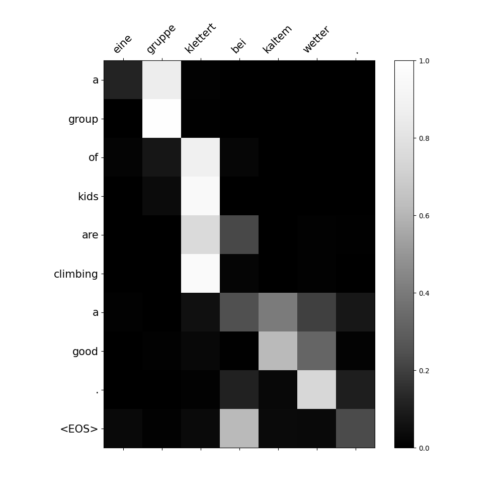
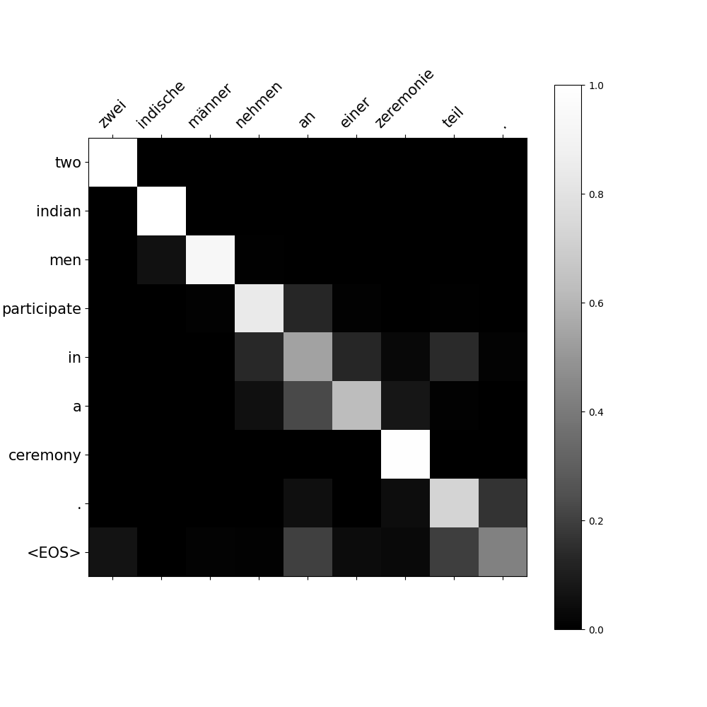
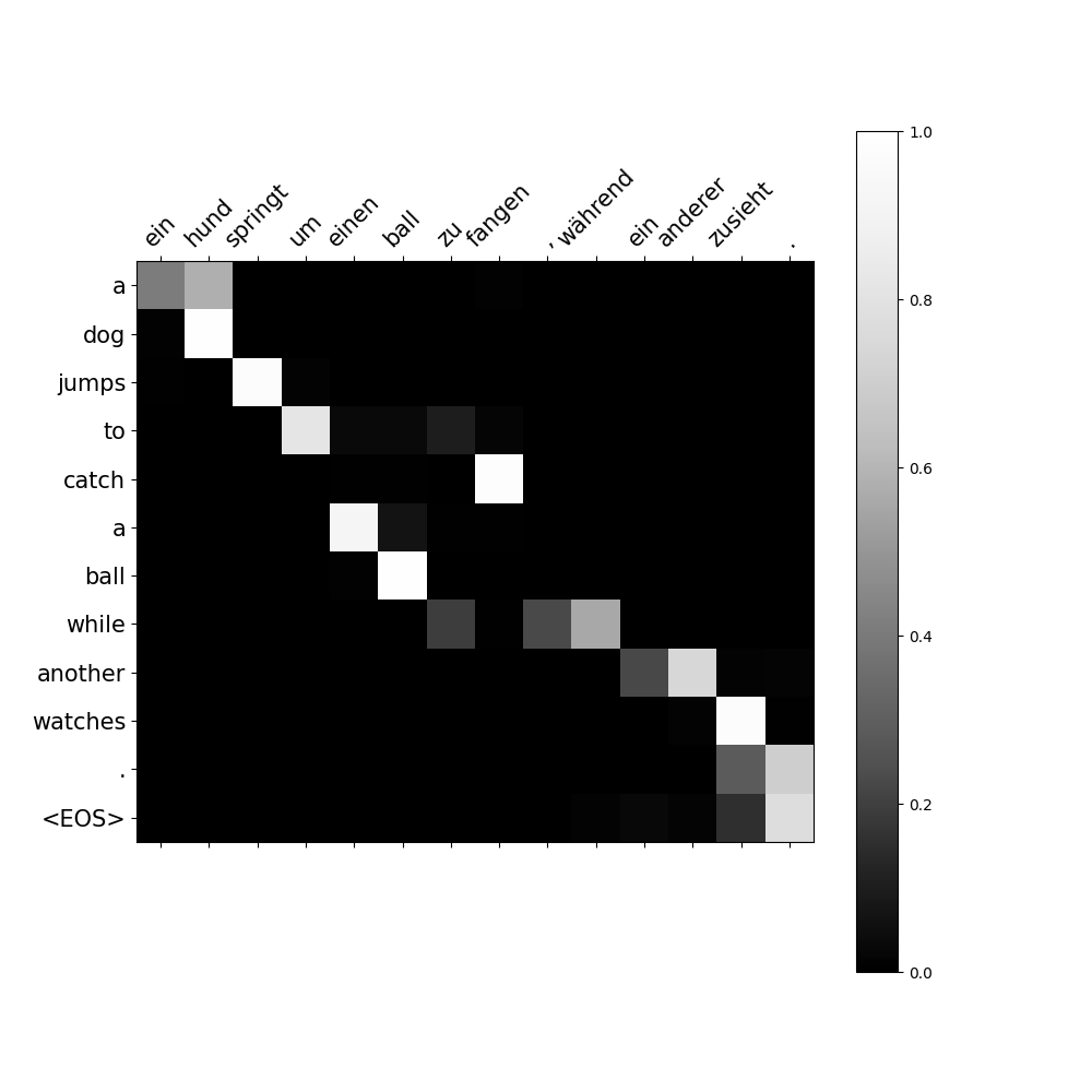
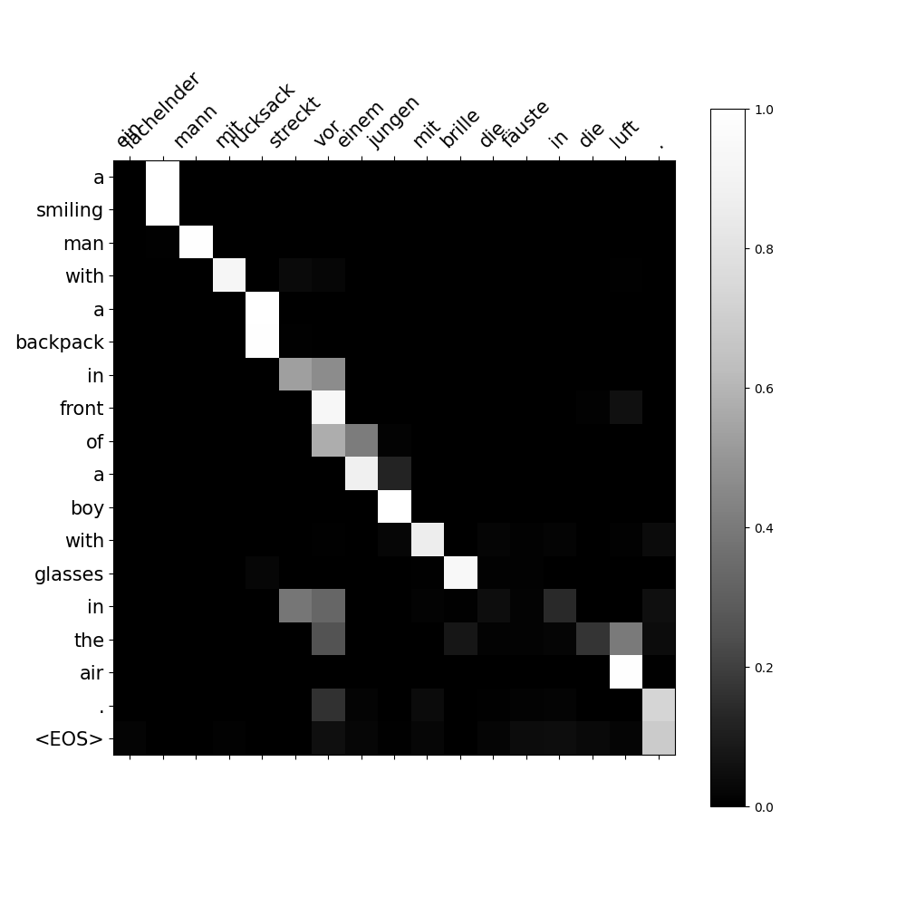
Off-diagonal weights can reflect word-order differences and multiword translations. These plots are useful diagnostics, but do not alone establish that the model has learned a particular grammatical rule.

Takeaways

• Selection and averaging claims need explicit assumptions about score gaps, masking, and scale.
• Consistent tensor layouts prevent confusion between batch and sequence axes.
• The recorded translation results favor attention in this experiment; stronger claims need matched settings and more runs.