Word Embeddings: PPMI, GloVe & Bias

Overview

This study uses AG News text to compare positive pointwise mutual information (PPMI) with dimensionality reduction and learned GloVe vectors. A separate analysis examines analogy outputs from pretrained word2vec embeddings.

The charts, training log, and analogy scores below come from the original experiment. They are not newly measured results.

Vocabulary and memory

The original report retained tokens occurring at least 12 times and reported approximately 96% token coverage. Coverage means the fraction of token occurrences represented, not the fraction of distinct word types.

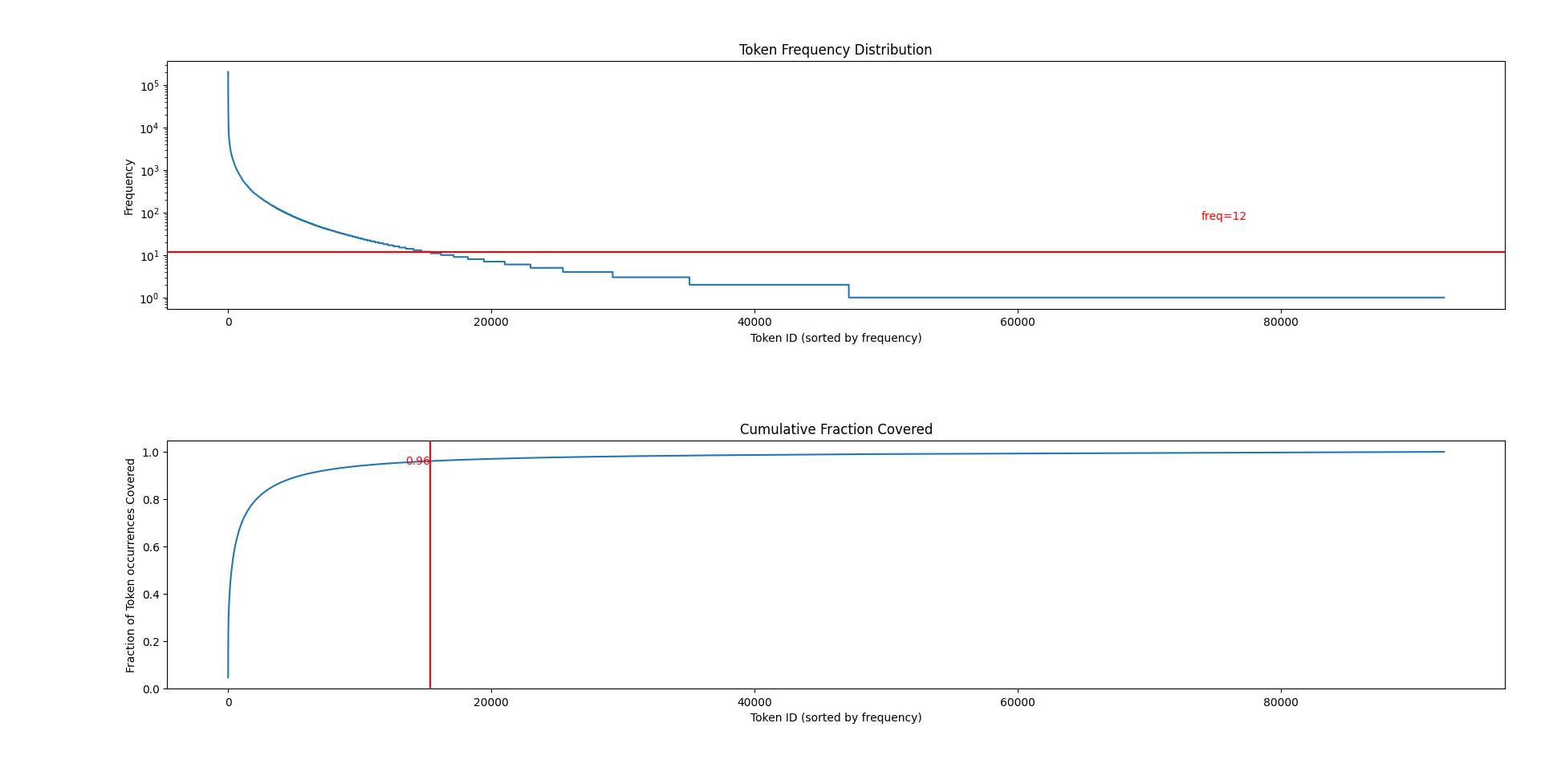
A dense co-occurrence matrix with vocabulary size $V$ requires $V^2b$ bytes, where $b$ is the number of bytes per entry. The earlier estimate of about 1 GB applies to that experiment's vocabulary and representation; it is not a general memory bound. Probability calculations and factorization can require additional copies.

Count-based vectors with PPMI

Let $C_{ij}$ count occurrences of word $i$ with context $j$, and let $N=\sum_{i,j}C_{ij}$. Estimate

$$P(i,j)=\frac{C_{ij}}{N},\quad P(i)=\frac{\sum_j C_{ij}}{N},\quad P(j)=\frac{\sum_i C_{ij}}{N}.$$

For positive joint and marginal probabilities,

$$\operatorname{PPMI}(i,j)= \max\left(0,\log\frac{P(i,j)}{P(i)P(j)}\right).$$

PPMI stands for positive pointwise mutual information. Zero-count pairs need explicit handling to avoid evaluating $\log 0$.

The repository computes $M\approx U_k\Sigma_kV_k^\top$, concatenates $U_k\Sigma_k^{1/2}$ and $V_k\Sigma_k^{1/2}$, and normalizes each row. With its default $k=16$, this produces 32-dimensional vectors before visualization.

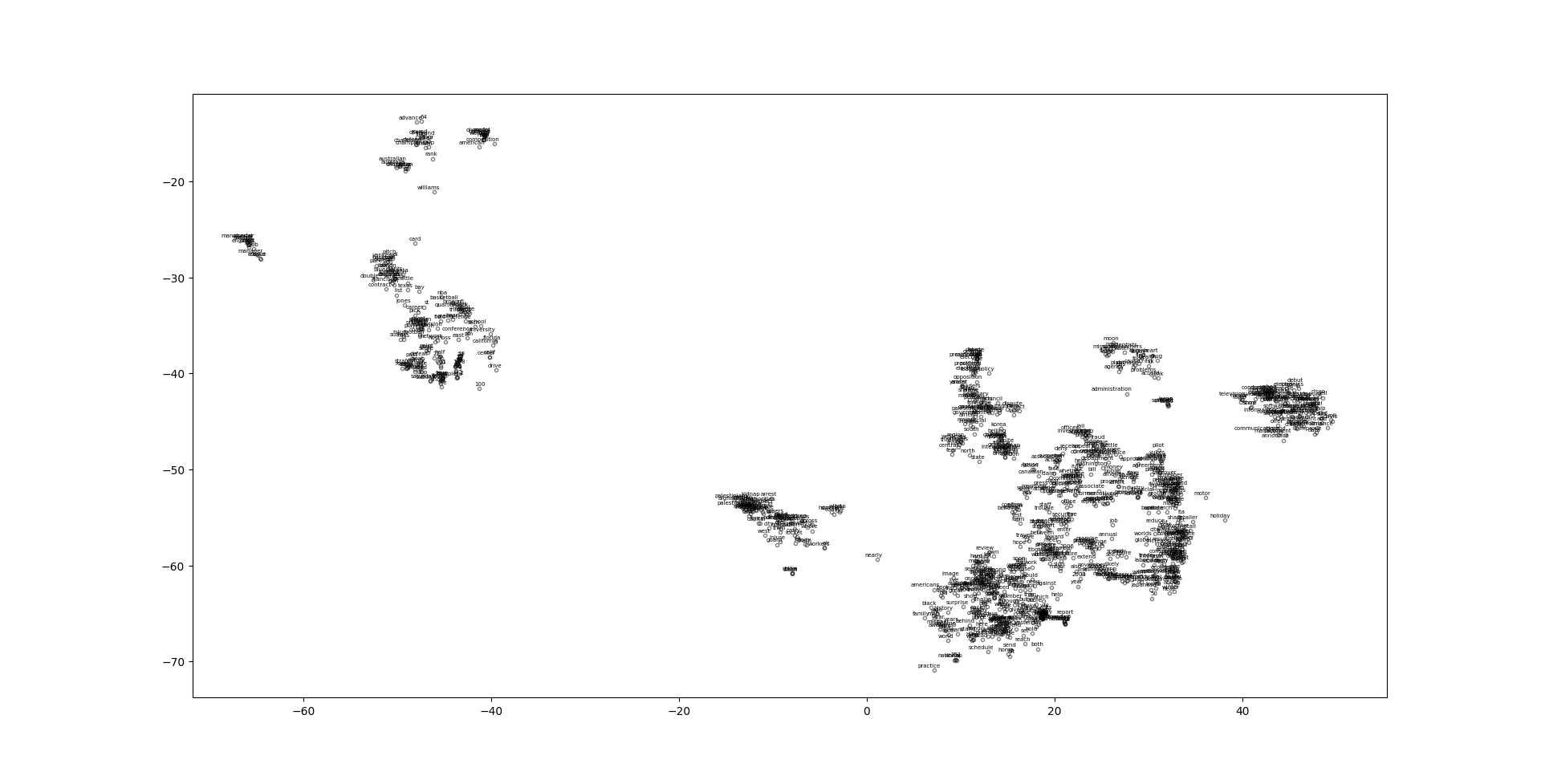
View the three topic close-ups

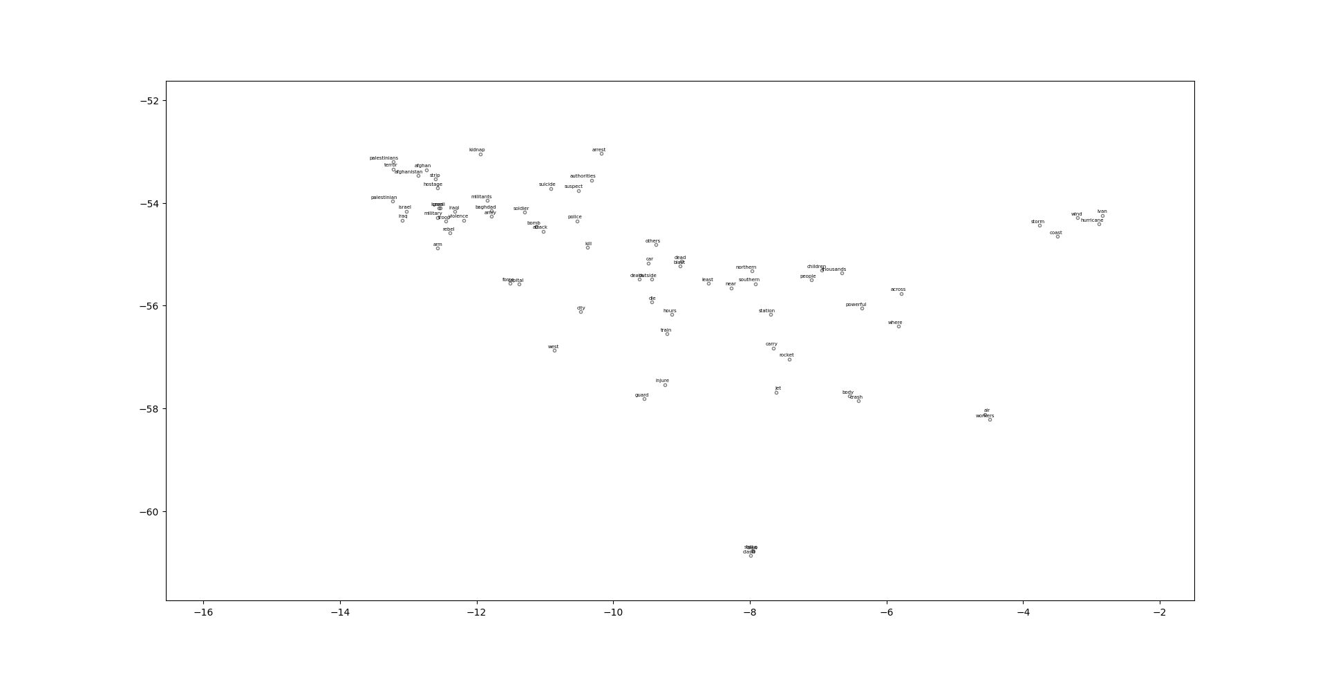
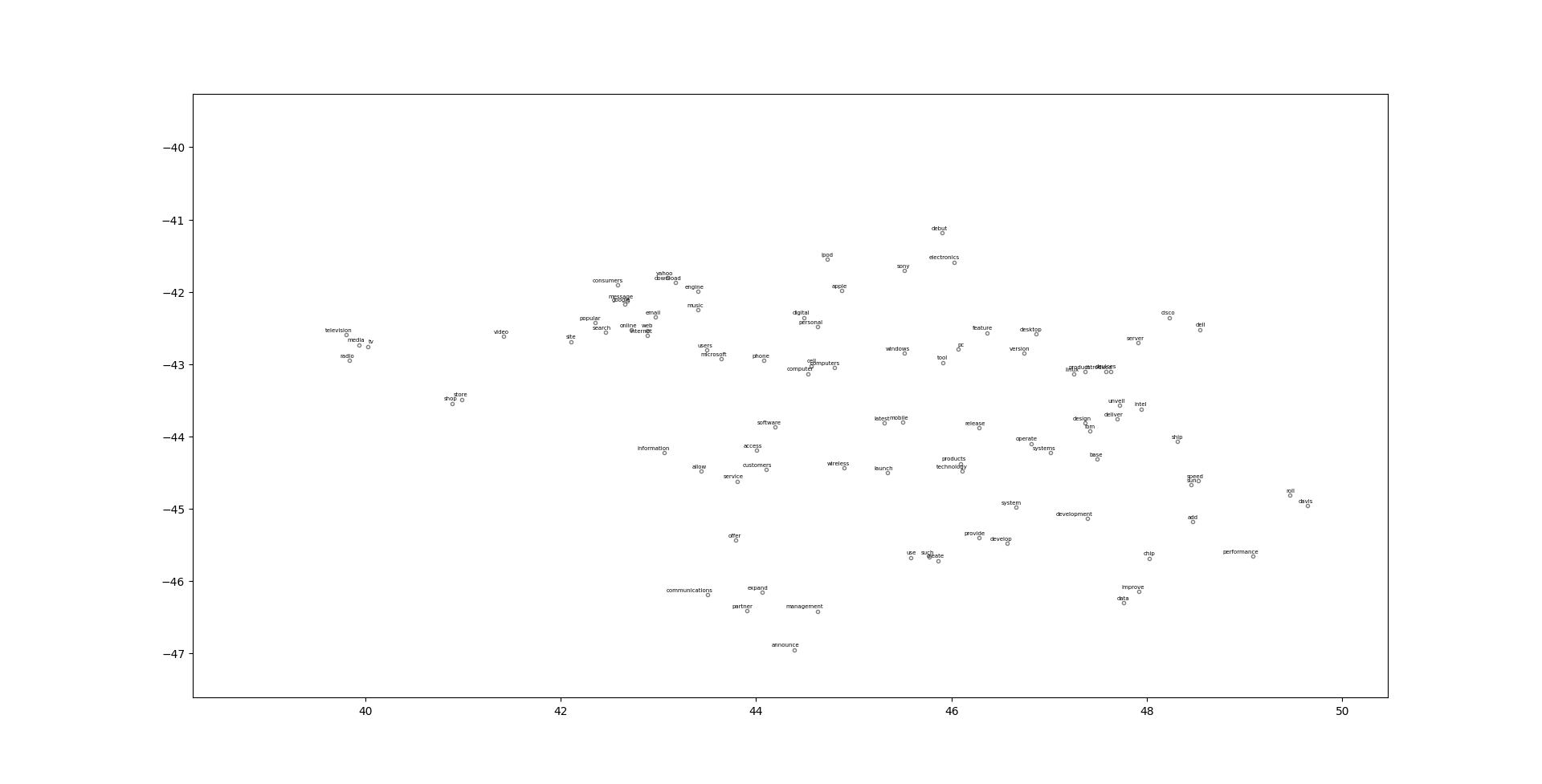
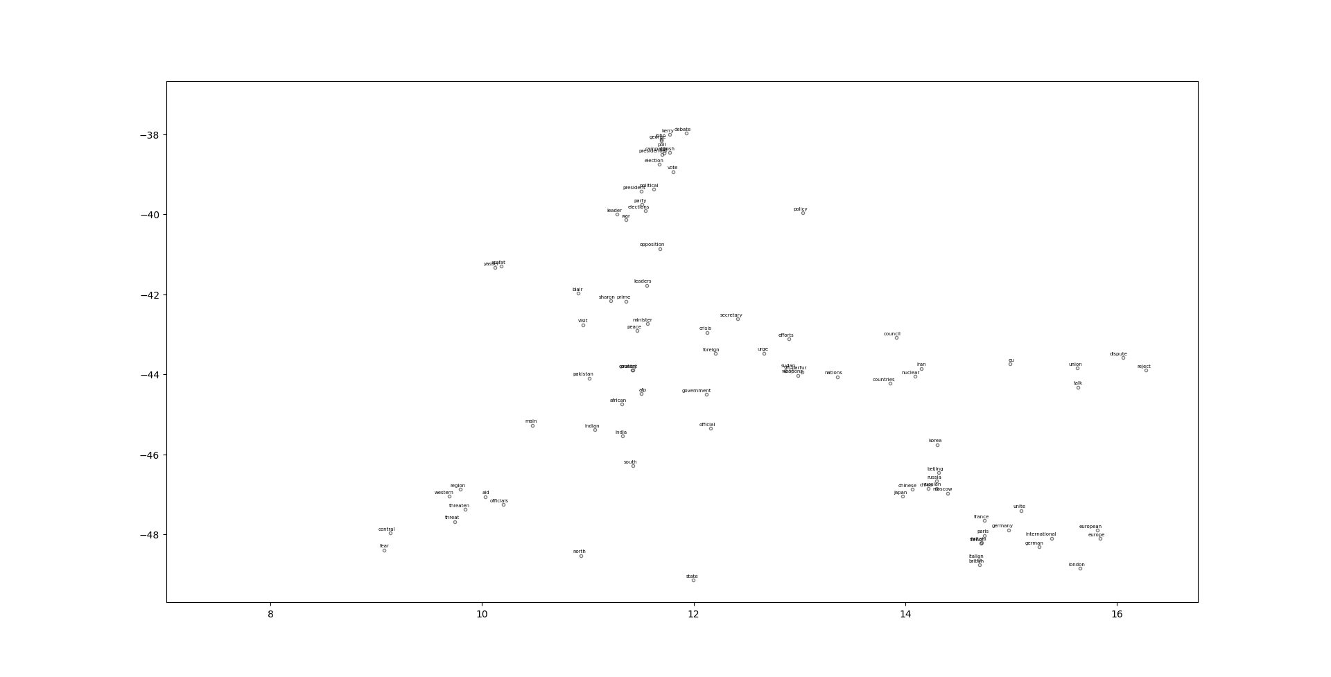
These views help inspect local neighborhoods. Distances between distant clusters, cluster sizes, and empty spaces in t-SNE should not be read as direct measurements of the original embedding geometry. See the t-SNE paper.

GloVe objective and gradients

For a pair with $C_{ij}>0$, define

$$e_{ij}=\mathbf w_i^\top\widetilde{\mathbf w}_j+b_i+\widetilde b_j-\log C_{ij}.$$

The objective and weighting function are

$$J=\sum_{i,j:C_{ij}>0}f(C_{ij})e_{ij}^2,\qquad f(x)=\min\left(1,\left(\frac{x}{x_{\max}}\right)^\alpha\right).$$

The implementation uses $x_{\max}=100$ and $\alpha=0.75$. Zero-count pairs are omitted. This weighted regression objective follows the GloVe paper.

One pair versus the full objective

For the single-pair loss $\ell_{ij}=f(C_{ij})e_{ij}^2$,

$$\begin{aligned} \nabla_{\mathbf w_i}\ell_{ij}&=2f(C_{ij})e_{ij}\widetilde{\mathbf w}_j,\\ \nabla_{\widetilde{\mathbf w}_j}\ell_{ij}&=2f(C_{ij})e_{ij}\mathbf w_i,\\ \frac{\partial\ell_{ij}}{\partial b_i} &=\frac{\partial\ell_{ij}}{\partial\widetilde b_j} =2f(C_{ij})e_{ij}. \end{aligned}$$

The full gradient must sum every contribution involving the parameter:

$$\nabla_{\mathbf w_i}J =\sum_{j:C_{ij}>0}2f(C_{ij})e_{ij}\widetilde{\mathbf w}_j.$$

The context-vector gradient sums over $i$; bias gradients sum over their respective partners. A minibatch implementation must accumulate repeated indices rather than overwrite their contributions.

Recorded training behavior

The final logged averages over 100 batches were approximately 0.0467–0.0483. This describes the end of the run; a short, stable loss segment alone does not establish convergence or downstream quality.

Iter 14400 / 15227: average loss = 0.046686563985831216
Iter 14700 / 15227: average loss = 0.04827717854832922
Iter 15200 / 15227: average loss = 0.04732485846561704

Interpreting analogy results

The separate word2vec analysis queried $\mathbf v_b-\mathbf v_a+\mathbf v_c$. The original nearest-neighbor outputs included:

These asymmetric associations motivate a broader bias evaluation. Scores measure vector similarity, not probabilities or facts about people. Two queries do not establish bias prevalence across the vocabulary or identify its cause. These pretrained word2vec results are separate from the AG News GloVe experiment.

Reproducing the study

The repository contains:

Record dependency versions, dataset, tokenizer, vocabulary cutoff, context definition, and random seed when comparing runs. The historical results have not been reproduced in a fresh training run.

Takeaways

• Coverage and memory depend on tokenization, cutoff, and storage format.
• Distinguish a pairwise gradient from the full gradient when implementing GloVe.
• Visualizations and analogy queries support exploration; general claims need broader evaluation.