Online Learning

Bandit Algorithms: Methods & Implementation Review

Compare exploration strategies and inspect where the experimental implementations differ from standard UCB, Thompson sampling, and nonlinear bandit methods.

Bandits

UCB

Thompson Sampling

Yong-Hwan Lee

Published October 20, 2023 · Updated September 29, 2026

Code

Overview

This Oregon State University study explores how bandit algorithms trade off collecting information and choosing actions with high estimated rewards. It covers independent-arm methods, linear contextual methods, and a squared-reward experiment.

The tables and figures preserve the original recorded results. A source review found differences between several implementations and their standard algorithm names. Those differences are explained alongside the results so that the numbers are interpreted as observations of the implemented variants.

Experiment and metric

For expected reward $\mu_t(i)$ and selected arm $A_t$ , cumulative pseudo-regret is

R_T=\sum_{t=1}^{T}\left[\max_{i\in\mathcal A_t}\mu_t(i)-\mu_t(A_t)\right].

The simulator adds the same sampled noise to the selected reward and the comparator reward, so that noise cancels in the recorded difference. With multiple users, its plotted cumulative regret is averaged across users.

The linked simulation's defaults are 25 context dimensions, 25 arms, 10 users, 200,000 iterations, and Gaussian observation noise with standard deviation 0.1. The archive does not pin a seed and complete configuration for every figure, so these defaults should not be assumed to describe every historical run.

A further logging detail matters: the source records every 100 iterations starting at zero and prints the last recorded point. That point need not equal the full-horizon total. The tables below retain the reported cumulative regret, rather than claiming a newly verified final-horizon result.

Explore-then-commit and UCB

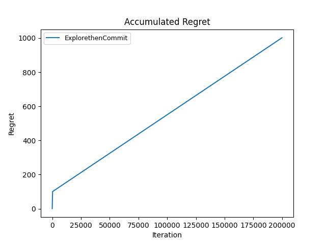
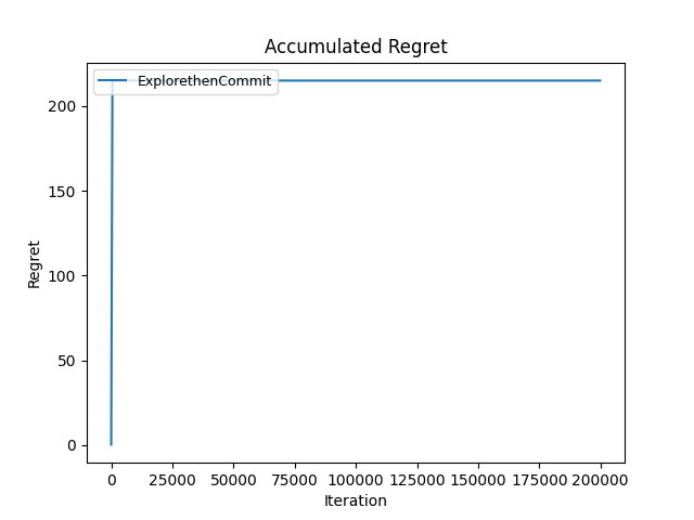
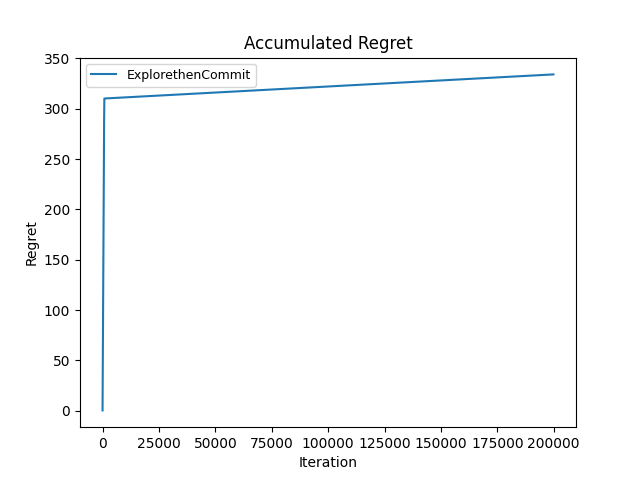
Explore-then-commit first gathers observations, then chooses the best empirical arm for the remaining rounds. Its exploration parameter $m$ controls the initial sampling budget. Too little exploration risks a poor commitment; more exploration also incurs a cost.

Explore-then-commit setting	Reported regret
$m=10$	1001.40
$m=20$	214.90
$m=30$	334.02

View explore-then-commit curves

UCB keeps exploring through a confidence bonus. For an arm with $N_i>0$ previous observations, the implementation uses

\operatorname{score}_t(i)=\widehat\mu_i+ \sqrt{\frac{2\alpha\log t}{N_i}},

where $t$ is the number of completed updates. Unobserved arms are selected before this expression is evaluated. The factor $\alpha$ was missing from the previous explanation, even though it changes the experiment.

UCB setting	Reported regret
$\alpha=0.1$	256.50
$\alpha=0.5$	977.03
$\alpha=1.0$	1906.65

View UCB curves

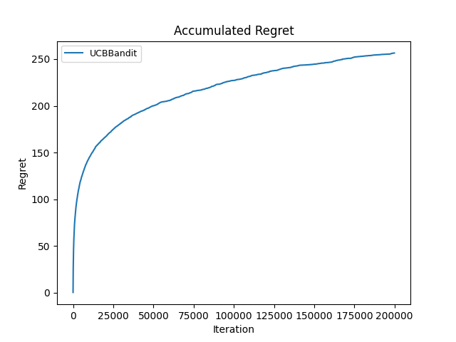
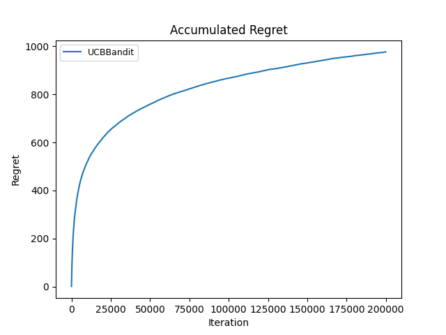
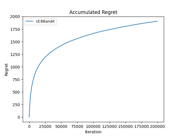
These runs show sensitivity to exploration settings. They do not establish that the smallest exploration bonus is generally best.

Gaussian reward sampling

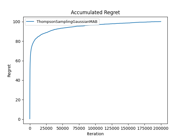
The class named ThompsonSamplingGaussianMAB draws an independent score for each arm using

np.random.normal(empirical_mean, 1 / (observation_count + 1))

NumPy's second argument is the standard deviation, not the variance. Therefore, the implemented score distribution is

\widetilde\mu_i\sim \mathcal N\left(\widehat\mu_i,\frac{1}{(N_i+1)^2}\right),

when the second parameter in $\mathcal N$ denotes variance.

The center is an empirical mean, and the shrinking scale is chosen directly in code. Without a corresponding prior and observation model, this is a Gaussian sampling heuristic rather than a derived Bayesian posterior update.

Archived method label	Reported regret
Thompson Sampling	100.00

View the Gaussian sampling curve

Gaussian sampling heuristic: cumulative regret

Linear contextual methods

With context vectors $x_s$ , observed rewards $r_s$ , and regularization $\lambda>0$ , define

A_t=\lambda I+\sum_{s<t}x_sx_s^\top,\qquad b_t=\sum_{s<t}x_sr_s,\qquad \widehat\theta_t=A_t^{-1}b_t.

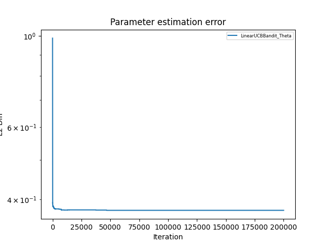
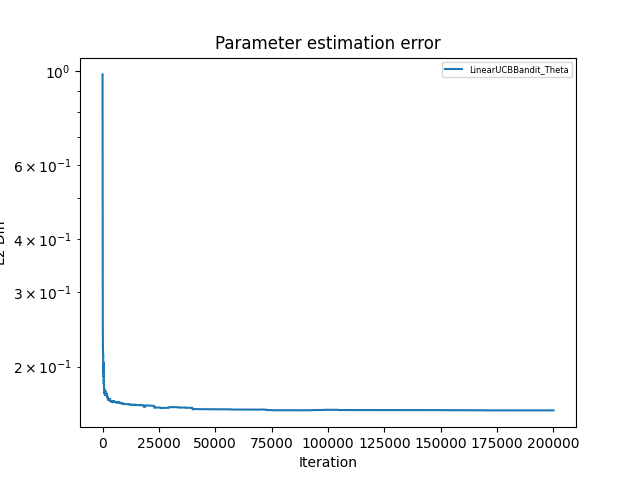
This is a regularized least-squares estimator for a linear reward model.

LinUCB

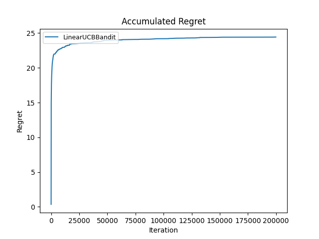
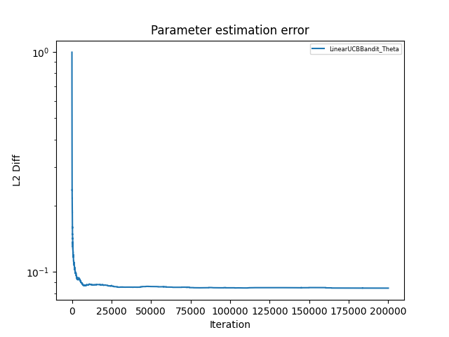
LinUCB evaluates an available context $x$ using

x^\top\widehat\theta_t+\alpha\sqrt{x^\top A_t^{-1}x}.

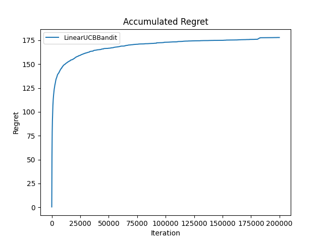
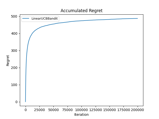
LinUCB setting	Reported regret
$\alpha=0.5$	24.43
$\alpha=1.5$	177.89
$\alpha=2.5$	487.73

View LinUCB regret and parameter error

Linear Thompson sampling

In a shared-parameter linear model, a standard Thompson decision samples one parameter vector,

\widetilde\theta_t\sim\mathcal N(\widehat\theta_t,v^2A_t^{-1}),

then scores every candidate with the same draw, $x^\top\widetilde\theta_t$ . The scale $v$ depends on the chosen posterior or exploration model.

The archived implementation samples inside the candidate-arm loop using covariance $A_t^{-1}$ . It therefore draws a different parameter vector for each candidate. That changes the joint distribution of arm scores and does not implement the shared-draw rule above.

Archived method label	Reported regret
Linear Thompson Sampling	1098.24

View the archived linear sampling curves

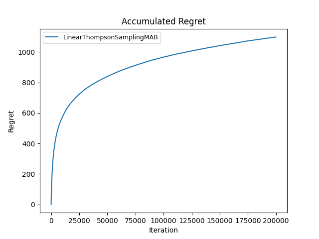
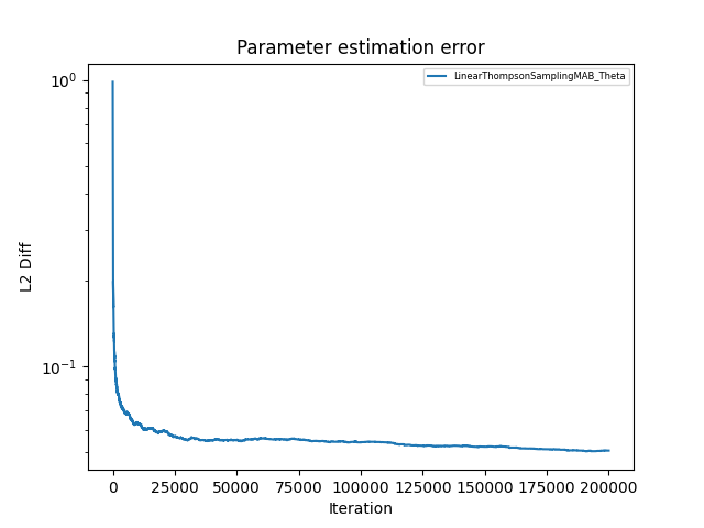
Per-arm parameter sampling: cumulative regret

Per-arm parameter sampling: parameter error

The figure remains useful as a record of that implementation. Its score should not be treated as a benchmark of the standard shared-parameter algorithm.

A nonlinear squared-reward experiment

The nonlinear simulator generates rewards of the form

r=(x^\top\theta)^2+\epsilon,\qquad \epsilon\sim\mathcal N(0,\sigma^2).

The archived GeneralizedLinearBandit class still estimates $\widehat\theta=A^{-1}b$ from linear sufficient statistics, then squares the prediction and adds a linear confidence bonus:

(x^\top\widehat\theta)^2+\alpha\sqrt{x^\top A^{-1}x}.

This is a squared-prediction heuristic, not a validated GLM-UCB implementation. In particular, $A^{-1}b$ is not the maximum-likelihood estimator for this nonlinear observation model. Under the stated Gaussian noise model, an unregularized maximum-likelihood fit instead minimizes

\sum_s\left[r_s-(x_s^\top\theta)^2\right]^2.

That objective is generally nonlinear and nonconvex. The squared link is not globally monotone and cannot distinguish $\theta$ from $-\theta$ , so parameter error against only one sign also needs care. Standard generalized-linear-bandit guarantees cannot simply be transferred to this experiment.

Squared-prediction heuristic setting	Reported regret
$\alpha=0.1$	62.16
$\alpha=0.5$	727.63
$\alpha=1.5$	5948.48

View the squared-reward experiment curves

Squared-reward heuristic regret, alpha = 0.1

Squared-reward heuristic regret, alpha = 0.5

Squared-reward heuristic regret, alpha = 1.5

Squared-reward heuristic parameter error, alpha = 0.1

Squared-reward heuristic parameter error, alpha = 0.5

Squared-reward heuristic parameter error, alpha = 1.5

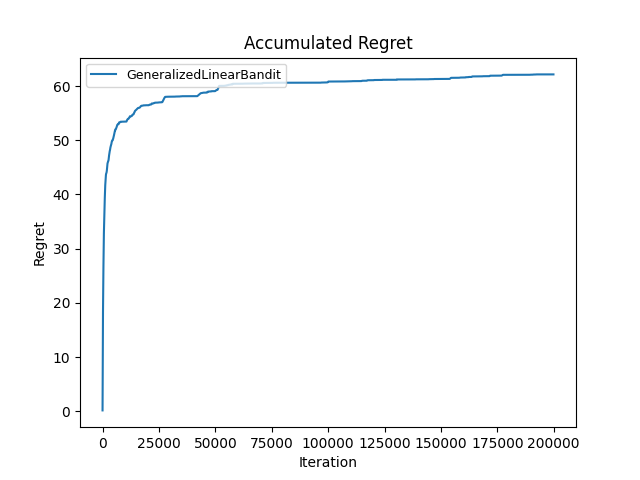
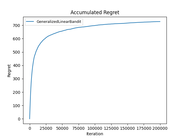
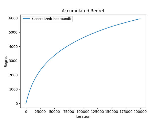
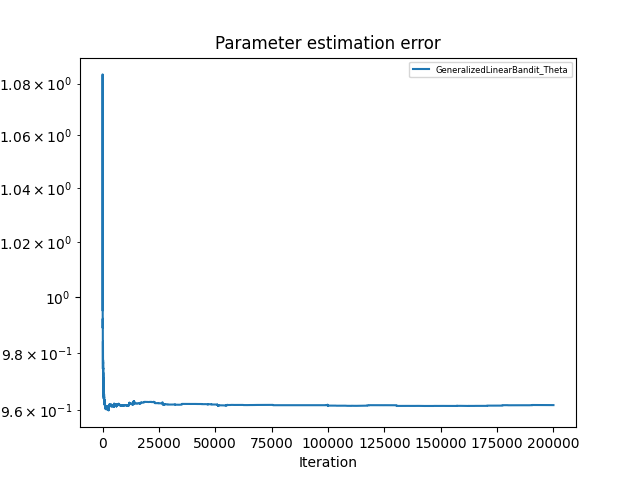
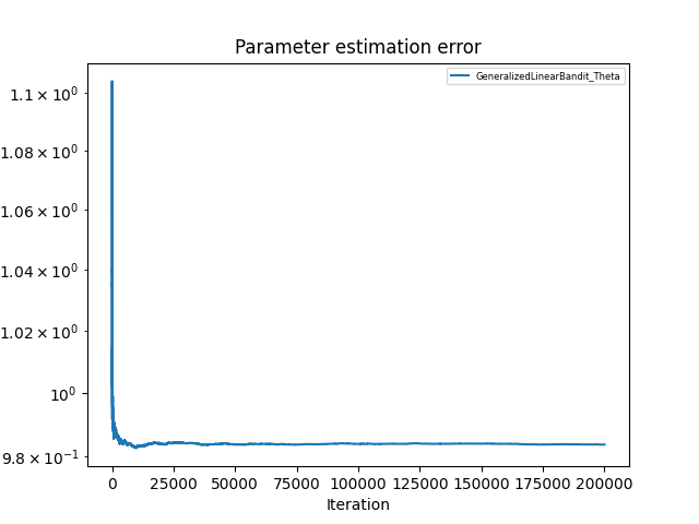
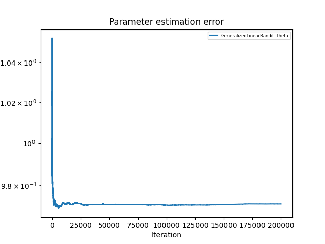
The original plots retain their historical “GLM-UCB” labels for traceability; the label does not resolve the estimator mismatch.

Reproduction notes

Use the repository's main branch. Simulation.py selects independent-arm and linear methods; SimulationNonLinear.py selects the nonlinear experiment. Algorithms are enabled in each script's algorithms dictionary.

Before making a new cross-algorithm comparison:

Fix environment settings and use matched random seeds across repeated runs.
Specify the actual sampling distribution, estimator, and confidence rule.
Record the full-horizon total in addition to periodic checkpoints.
Report a mean and uncertainty across runs, separately for each reward model.

No training or simulation results were regenerated during this content review. The external repository's implementations remain unchanged.

Takeaways

Exploration settings can dominate a single run; one regret value does not determine an algorithm ranking.
Standard deviation, covariance, and shared parameter draws change the algorithm being evaluated.
A nonlinear prediction formula does not make a linear estimator a nonlinear maximum-likelihood estimator.
Reading the implementation is necessary to interpret the experiment's labels and metrics.